FlashAttention in Triton: A Tile-by-Tile Walkthrough

In my TurboQuant kernel, I computed attention scores. This time, I wanted to finish the operation: turn those scores into weights and use them to combine information.

Writing the equation was easy. Understanding why FlashAttention rearranges the work took longer. The breakthrough was realizing that a GPU can compute an intermediate result without saving the entire matrix it belongs to.

First, what does attention actually do?

Imagine reading a sentence and deciding which other words help explain the current word. Attention makes a numerical version of that decision. The model learns three representations:

• A query describes what a position is looking for.
• A key describes what another position can match.
• A value contains the information that position contributes.

Compare a query with every key using dot products. Divide the scores by sqrt(D) to control their scale. Softmax then turns them into positive weights that sum to one. Finally, use those weights to average the value vectors:

Softmax operates on each query's row. Q contains M query rows; K and V contain N rows each. In this implementation, all vectors have D features, so the output O has shape M × D.

That is ordinary attention. FlashAttention changes how we carry it out on the GPU.

The expensive part is saving the middle

A straightforward implementation writes the full M × N score matrix S to GPU memory, reads it for softmax, writes the probability matrix P, then reads that for the multiplication by V.

This memory is called HBM, the GPU's large off-chip memory. Moving data between HBM and the smaller, faster on-chip working storage costs time. At M=1024 and N=4096, one FP32 score matrix takes 16 MiB. Separate full S and P arrays would take 32 MiB, before inputs and outputs.

The FlashAttention paper asks a useful question: can we consume each small piece of those matrices immediately, instead of saving the whole thing?

Yes. Keep a tile of queries, bring in a tile of keys and values, compute their scores, and immediately update a compact running result. Repeat until every key has been visited. This combines tiling, fused computation, and online softmax.

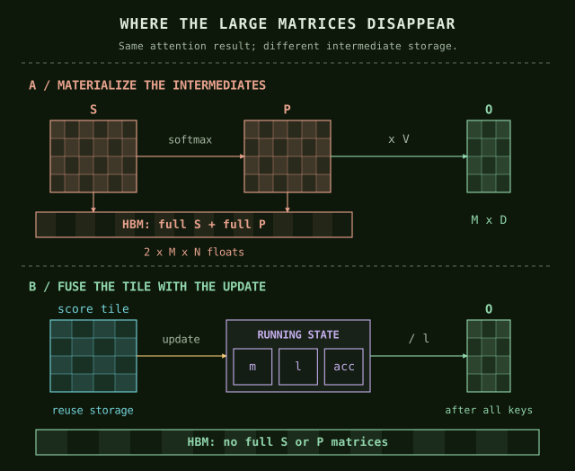
This is still dense attention: every query meets every key, and the arithmetic remains quadratic in sequence length. The saving comes from avoiding full intermediate matrices and their memory traffic. The mathematical result is unchanged; floating-point rounding can differ. The upper path above illustrates materialized attention, rather than the internals of a particular PyTorch backend.

How can softmax work a tile at a time?

This was the part I had to slow down for. A softmax weight depends on all the scores in its row. Normalizing each tile separately would give several unrelated denominators and the wrong answer.

Instead, keep three things per query:

• m: the largest score seen so far.
• l: the sum of exponentials, measured relative to m.
• acc: the weighted sum of value vectors, on that same scale.

Subtracting the maximum before exponentiation prevents large positive scores from overflowing. If a later tile raises the maximum, adjust the earlier contributions to the new scale.

Take already-scaled scores [1, 2, 3] with scalar values [10, 20, 30]. After reading the first two scores, the maximum is 2. Their unnormalized weights are exp(1-2) and exp(2-2), approximately [0.368, 1].

Now score 3 arrives. The new maximum is 3. Multiply both old weights by exp(2-3), giving [0.135, 0.368], then add the new weight 1. All three contributions now share the same reference point:

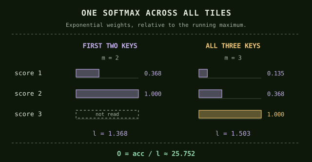
We do not actually keep those earlier weights. Multiplying their sum l and weighted accumulator acc by the same factor has exactly the required effect. Here, the final denominator is about 1.503 and the weighted sum is 38.711. Divide once at the end to get 25.752.

For a new tile of scaled scores s, that idea becomes:

Here a is acc, and p contains unnormalized weights. Start with m=-inf, l=0, and acc=0; write acc / l after the last tile. The tiny example uses blocks of two and one keys, while my kernel uses blocks of 16.

Now map the idea to Triton

A Triton program is a cooperative GPU work unit. My launch assigns 16 query rows to each program. It loads those queries once, then streams through matching 16-row key and value tiles.

The highlighted bands below are whole tiles. Q_i stays fixed while K_j and V_j advance together. Each pair of query and key tiles produces a 16 × 16 score tile:

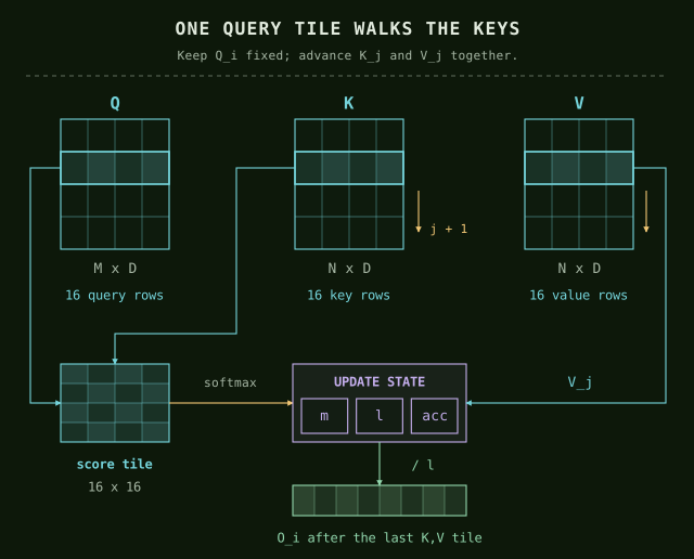
The implementation follows that picture:

1. tl.load reads the query tile before the loop, then the current key and value tiles inside it.
2. tl.dot(q, tl.trans(k)) computes scores. The m_new, alpha, and l_new updates implement the recurrence above; tl.dot(p, v, acc) adds the weighted values.
3. After the loop, tl.store writes acc / l to the output.

There are ceil(M / 16) programs. Features are padded to max(16, next_power_of_2(D)), and masks exclude padding. This first version handles contiguous two-dimensional FP32 tensors with one head. It has no causal mask, dropout, batch dimension, or backward implementation.

Full Triton implementation

This is the complete reviewed source, including the launch wrapper. Use Copy code, or download the Python file.

1
2
3
4
5
6
7
8
9
10
11
12
13
14
15
16
17
18
19
20
21
22
23
24
25
26
27
28
29
30
31
32
33
34
35
36
37
38
39
40
41
42
43
44
45
46
47
48
49
50
51
52
53
54
55
56
57
58
59
60
61
62
63
64
65
66
67
68
69
70
71
72
73
74
75
76
77
78
79
80
81
82
83
84
85
86
87
88
89
90
91
92
93
94
95
96
97
98
99
100
101
102
103
104
105
106
107
108
109
110
111
112
113
114
115
116
117
118
119
120
121
122
123
124
125
126
127
128
129
130
131
132
133
134
135
136
137
138
139

import torch
import triton
import triton.language as tl


@triton.jit
def flash_attention_fwd_kernel(
    Q_ptr, K_ptr, V_ptr, out_ptr,
    M, N, D, scale,
    BLOCK_M: tl.constexpr,
    BLOCK_N: tl.constexpr,
    BLOCK_DMODEL: tl.constexpr,
):
    # Each program handles a group of query rows.
    pid_m = tl.program_id(0)

    # Indices of the query rows handled by this program.
    offs_m = pid_m * BLOCK_M + tl.arange(0, BLOCK_M)

    # Feature indices. Extra positions are padded with zeros.
    offs_d = tl.arange(0, BLOCK_DMODEL)

    # Indices used to load K and V in chunks.
    offs_n = tl.arange(0, BLOCK_N)

    # Load Q once and reuse it while processing all K/V blocks.
    q = tl.load(
        Q_ptr + offs_m[:, None] * D + offs_d[None, :],
        mask=(offs_m[:, None] < M) &
             (offs_d[None, :] < D),
        other=0.0
    )

    # Online softmax state:
    # m_i = maximum attention score seen so far.
    # l_i = running sum of exponentials.
    # acc = running weighted sum of V.
    m_i = tl.full((BLOCK_M,), float("-inf"), tl.float32)
    l_i = tl.zeros((BLOCK_M,), dtype=tl.float32)
    acc = tl.zeros((BLOCK_M, BLOCK_DMODEL), dtype=tl.float32)

    # Process all key/value rows in smaller blocks.
    for start_n in range(tl.cdiv(N, BLOCK_N)):

        cols_n = start_n * BLOCK_N + offs_n

        # Load the current key block.
        k = tl.load(
            K_ptr + cols_n[:, None] * D + offs_d[None, :],
            mask=(cols_n[:, None] < N) &
                 (offs_d[None, :] < D),
            other=0.0
        )

        # Load the corresponding value block.
        v = tl.load(
            V_ptr + cols_n[:, None] * D + offs_d[None, :],
            mask=(cols_n[:, None] < N) &
                 (offs_d[None, :] < D),
            other=0.0
        )

        # Calculate attention scores for the current Q/K block.
        qk = tl.dot(q, tl.trans(k), input_precision="ieee")
        qk = qk * scale

        # Ignore padded key columns and padded query rows.
        qk = tl.where(cols_n[None, :] < N, qk, float("-inf"))
        qk = tl.where(offs_m[:, None] < M, qk, float("-inf"))

        # Find the maximum score in the current block.
        m_ij = tl.max(qk, axis=1)

        # Update the maximum across all blocks processed so far.
        m_new = tl.maximum(m_i, m_ij)

        # Rescale previous results if the maximum has changed.
        alpha = tl.exp(m_i - m_new)

        # Calculate exponentials for the current block.
        p = tl.exp(qk - m_new[:, None])

        # Update the running softmax denominator.
        l_new = alpha * l_i + tl.sum(p, axis=1)

        # Rescale the previous weighted output.
        acc = acc * alpha[:, None]

        # Add weighted values from the current block.
        acc = tl.dot(p, v, acc, input_precision="ieee")

        # Save the updated online softmax state.
        m_i = m_new
        l_i = l_new

    # Normalize the accumulated weighted values.
    out = acc / l_i[:, None]

    # Store only the actual query rows and feature dimensions.
    tl.store(
        out_ptr + offs_m[:, None] * D + offs_d[None, :],
        out,
        mask=(offs_m[:, None] < M) &
             (offs_d[None, :] < D)
    )


def solve(
    Q: torch.Tensor,
    K: torch.Tensor,
    V: torch.Tensor,
    out: torch.Tensor
) -> None:

    # M = number of query rows.
    # N = number of key/value rows.
    # D = feature dimension.
    M, D = Q.shape
    N = K.shape[0]

    scale = 1.0 / (D ** 0.5)

    BLOCK_M = 16
    BLOCK_N = 16

    # tl.dot requires a reduction dimension of at least 16.
    BLOCK_DMODEL = max(16, triton.next_power_of_2(D))

    # One program handles BLOCK_M query rows.
    grid = (triton.cdiv(M, BLOCK_M),)

    flash_attention_fwd_kernel[grid](
        Q, K, V, out,
        M, N, D, scale,
        BLOCK_M=BLOCK_M,
        BLOCK_N=BLOCK_N,
        BLOCK_DMODEL=BLOCK_DMODEL,
        num_warps=4
    )

To reproduce the benchmark from the repository:

modal run benchmarks/sm90/fp32/h100/flash_attention_triton.py

The benchmark harness contains the reference and timing procedure. For a more advanced implementation, the official Triton fused-attention tutorial is a useful next read.

What the H100 run showed

My saved Modal run used an NVIDIA H100 80GB, CUDA 12.4, PyTorch 2.4.0, and Triton 3.0.0. The README at commit 682118f agrees with the saved benchmark JSON. I have not rerun the GPU benchmark for this article.

All three correctness cases passed against explicit softmax(Q @ K.T / sqrt(D)) @ V, including odd sizes (7,13,8), (35,67,32), and (64,129,128). The largest absolute error was 3.13e-7, with rtol=2e-3 and atol=2e-3.

The latency comparison uses PyTorch's scaled_dot_product_attention API. Timings below are converted from milliseconds to microseconds; lower is better.

That is nearly level on the smallest case and about 1.9 times slower on the larger two. The harness uses CUDA-event averages after ten warmups, with 100, 50, and 20 timed iterations respectively. Triton writes a preallocated output; SDPA returns a new tensor. The selected SDPA backend was not recorded, so these numbers are an API comparison, not evidence of beating or matching the official FlashAttention implementation.

At the largest shape, my launch has just 64 query programs, each visiting 256 key/value tiles. The GPU has 132 SMs. I would next measure different tile sizes and ways to expose more parallel work, while retaining the precision and correctness checks. This kernel fixes both tile sizes at 16 and uses input_precision="ieee"; it has no autotuning.

What I took from this version is a distinction I want to keep measuring: avoiding a large intermediate is an algorithmic improvement; achieving the fastest kernel takes further work on scheduling, precision, and data movement.